library("MASS")
set.seed(123456)


### building a toy data set ###

## number of observations
n <- 500

## good predictor
good_x <- rnorm(n = n, mean = 0.5, sd = 1)

## noisy variable, which is highly correlated with good predictor
noisy_x <- good_x + rnorm(n, mean = 0, sd = 1.2)

## response variable linear to good_x plus random error
y <- 0.7 * good_x + rnorm(n, mean = 0, sd = 0.11)

## variables with no relation to response 10 variables, 5 are always
## correlated
Sigma_diag <- matrix(0.6, nrow = 5, ncol = 5)
zeros <- matrix(0, nrow = 5, ncol = 5)
Sigma <- rbind(cbind(Sigma_diag, zeros), cbind(zeros, Sigma_diag))
diag(Sigma) <- 1
random_X <- mvrnorm(n = n, mu = rep(0, 10), Sigma = Sigma)
colnames(random_X) <- paste("useless", 1:10, sep = "_")

## binding all together
dat <- data.frame(y = y, good_x, noisy_x, random_X)

## relationship between y and good_x and noisy_x
par(mfrow = c(1, 2))
plot(y ~ good_x, data = dat)
plot(y ~ noisy_x, data = dat)

## pca
prin <- princomp(dat[-1], cor = TRUE)

## results visualized
par(mfrow = c(1, 2))
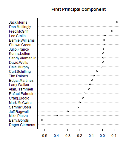
screeplot(prin, type = "l")

loadings(prin)

## 
## Loadings:
##            Comp.1 Comp.2 Comp.3 Comp.4 Comp.5 Comp.6 Comp.7 Comp.8 Comp.9
## good_x                    0.700  0.148                0.459        -0.441
## noisy_x                   0.700         0.148        -0.424         0.474
## useless_1  -0.183 -0.408        -0.290        -0.464  0.382 -0.184  0.180
## useless_2  -0.204 -0.390         0.170  0.490  0.549  0.114        -0.116
## useless_3  -0.228 -0.393         0.242        -0.434         0.176       
## useless_4  -0.201 -0.394        -0.446 -0.278  0.309 -0.103  0.599       
## useless_5  -0.172 -0.414         0.365 -0.271  0.105 -0.306 -0.484       
## useless_6   0.413 -0.172         0.209 -0.527        -0.125              
## useless_7   0.411 -0.171        -0.305         0.273  0.398 -0.311  0.413
## useless_8   0.368 -0.241        -0.424  0.340 -0.252 -0.403 -0.209 -0.447
## useless_9   0.398 -0.191         0.366  0.386 -0.166         0.427  0.262
## useless_10  0.405 -0.215         0.137 -0.157  0.122               -0.297
##            Comp.10 Comp.11 Comp.12
## good_x     -0.234           0.146 
## noisy_x     0.239                 
## useless_1   0.144  -0.440  -0.252 
## useless_2   0.272  -0.284   0.196 
## useless_3   0.264   0.561   0.347 
## useless_4  -0.237                 
## useless_5  -0.443          -0.220 
## useless_6   0.186  -0.392   0.515 
## useless_7           0.412   0.165 
## useless_8  -0.135           0.150 
## useless_9  -0.416  -0.166  -0.171 
## useless_10  0.484   0.212  -0.596 
## 
##                Comp.1 Comp.2 Comp.3 Comp.4 Comp.5 Comp.6 Comp.7 Comp.8
## SS loadings     1.000  1.000  1.000  1.000  1.000  1.000  1.000  1.000
## Proportion Var  0.083  0.083  0.083  0.083  0.083  0.083  0.083  0.083
## Cumulative Var  0.083  0.167  0.250  0.333  0.417  0.500  0.583  0.667
##                Comp.9 Comp.10 Comp.11 Comp.12
## SS loadings     1.000   1.000   1.000   1.000
## Proportion Var  0.083   0.083   0.083   0.083
## Cumulative Var  0.750   0.833   0.917   1.000

dat_pca <- as.data.frame(prin$scores)
dat_pca$y <- y

plot(y ~ Comp.3, data = dat_pca)

## linear model detects good_x rightfully as only good significant
## predictor
mod <- lm(y ~ ., dat)
summary(mod)

## 
## Call:
## lm(formula = y ~ ., data = dat)
## 
## Residuals:
##     Min      1Q  Median      3Q     Max 
## -0.3205 -0.0750 -0.0048  0.0784  0.3946 
## 
## Coefficients:
##              Estimate Std. Error t value Pr(>|t|)    
## (Intercept) -0.001377   0.005681   -0.24     0.81    
## good_x       0.705448   0.006411  110.03   <2e-16 ***
## noisy_x     -0.002980   0.004288   -0.70     0.49    
## useless_1   -0.010783   0.006901   -1.56     0.12    
## useless_2    0.009326   0.006887    1.35     0.18    
## useless_3   -0.001307   0.007572   -0.17     0.86    
## useless_4   -0.005631   0.007037   -0.80     0.42    
## useless_5    0.002154   0.007116    0.30     0.76    
## useless_6   -0.001407   0.007719   -0.18     0.86    
## useless_7   -0.003830   0.007513   -0.51     0.61    
## useless_8    0.004877   0.007215    0.68     0.50    
## useless_9    0.000769   0.007565    0.10     0.92    
## useless_10   0.005247   0.007639    0.69     0.49    
## ---
## Signif. codes:  0 '***' 0.001 '**' 0.01 '*' 0.05 '.' 0.1 ' ' 1 
## 
## Residual standard error: 0.112 on 487 degrees of freedom
## Multiple R-squared: 0.976,   Adjusted R-squared: 0.975 
## F-statistic: 1.62e+03 on 12 and 487 DF,  p-value: <2e-16 
## 

dat_pca_reduced <- dat_pca[c 1=""Comp.1"," 2=""Comp.2"," 3=""Comp.3"," 4=""Comp.4")" language="("y","][/c]
mod_pca_reduced <- lm(y ~ ., data = dat_pca_reduced)

summary(mod_pca_reduced)

## 
## Call:
## lm(formula = y ~ ., data = dat_pca_reduced)
## 
## Residuals:
##     Min      1Q  Median      3Q     Max 
## -0.9634 -0.2188 -0.0147  0.2084  0.9651 
## 
## Coefficients:
##             Estimate Std. Error t value Pr(>|t|)    
## (Intercept)  0.35828    0.01463   24.50  < 2e-16 ***
## Comp.1       0.03817    0.00786    4.86  1.6e-06 ***
## Comp.2      -0.00778    0.00795   -0.98     0.33    
## Comp.3       0.48733    0.01149   42.41  < 2e-16 ***
## Comp.4       0.11190    0.02138    5.24  2.4e-07 ***
## ---
## Signif. codes:  0 '***' 0.001 '**' 0.01 '*' 0.05 '.' 0.1 ' ' 1 
## 
## Residual standard error: 0.327 on 495 degrees of freedom
## Multiple R-squared: 0.789,   Adjusted R-squared: 0.787 
## F-statistic:  463 on 4 and 495 DF,  p-value: <2e-16 
## 

library("randomForest")

## raw data
set.seed(1234)
forest <- randomForest(y ~ ., data = dat)
forest

## 
## Call:
##  randomForest(formula = y ~ ., data = dat) 
##                Type of random forest: regression
##                      Number of trees: 500
## No. of variables tried at each split: 4
## 
##           Mean of squared residuals: 0.03436
##                     % Var explained: 93.15

## pca data
set.seed(1234)
forest_pca <- randomForest(y ~ ., data = dat_pca)
forest_pca

## 
## Call:
##  randomForest(formula = y ~ ., data = dat_pca) 
##                Type of random forest: regression
##                      Number of trees: 500
## No. of variables tried at each split: 4
## 
##           Mean of squared residuals: 0.07293
##                     % Var explained: 85.47

## reduced pca data
set.seed(1234)
forest_pca <- randomForest(y ~ ., data = dat_pca_reduced)
forest_pca

## 
## Call:
##  randomForest(formula = y ~ ., data = dat_pca_reduced) 
##                Type of random forest: regression
##                      Number of trees: 500
## No. of variables tried at each split: 1
## 
##           Mean of squared residuals: 0.1456
##                     % Var explained: 70.98

My amazing, awesome wife often comes up with the little puzzles for our amazing children, and this one seemed destined to be solved in R. So, using up to 5 coins (1p, 2p, 5p, 10p, 20p and 50p) first she asked our
kids whether they could make every value up to 50p, and then what the smallest value they couldn't make was.

Here's my R solution (which took about 5mins less than our daughter took to answer the first question)

# What Amounts can't you make using up to 5 coins 1p to 50p
# 
# Author: Paul Hurley
library(ggplot2)
library(plyr)
# Define our coins
coins <- as.factor(c(0, 1, 2, 5, 10, 20, 50))
# build a list of all the possibilities
possibilities <- expand.grid(coin1 = coins, coin2 = coins, coin3 = coins, coin4 = coins, 
    coin5 = coins)
# calculate the result
possibilities$total <- as.numeric(as.character(possibilities$coin1)) + as.numeric(as.character(possibilities$coin2)) + 
    as.numeric(as.character(possibilities$coin3)) + as.numeric(as.character(possibilities$coin4)) + 
    as.numeric(as.character(possibilities$coin5))
# define our target values
targets <- 1:250
# what amounts aren't possible
targets[!targets %in% possibilities$total]

##  [1]  88  89  98  99 118 119 128 129 133 134 136 137 138 139 143 144 146
## [18] 147 148 149 158 159 163 164 166 167 168 169 173 174 176 177 178 179
## [35] 181 182 183 184 185 186 187 188 189 191 192 193 194 195 196 197 198
## [52] 199 203 204 206 207 208 209 211 212 213 214 215 216 217 218 219 221
## [69] 222 223 224 225 226 227 228 229 230 231 232 233 234 235 236 237 238
## [86] 239 240 241 242 243 244 245 246 247 248 249

So, the smallest value we can't make is
88

We can even produce a table of the number of ways to make each
number, and a graph

tableofpossibilities <- ddply(.data = possibilities, .(total), nrow)
ggplot(data = possibilities, aes(x = total)) + geom_histogram(binwidth = 1)

Then when I triumphantly told her, she asked, 'what about 4 coins ?'

# How about 4 coins build a list of all the possibilities
fourpossibilities <- expand.grid(coin1 = coins, coin2 = coins, coin3 = coins, 
    coin4 = coins)
# calculate the result
fourpossibilities$total <- as.numeric(as.character(fourpossibilities$coin1)) + 
    as.numeric(as.character(fourpossibilities$coin2)) + as.numeric(as.character(fourpossibilities$coin3)) + 
    as.numeric(as.character(fourpossibilities$coin4))
# what values can't be made ?
targets[!targets %in% fourpossibilities$total]

##   [1]  38  39  48  49  68  69  78  79  83  84  86  87  88  89  93  94  96
##  [18]  97  98  99 108 109 113 114 116 117 118 119 123 124 126 127 128 129
##  [35] 131 132 133 134 135 136 137 138 139 141 142 143 144 145 146 147 148
##  [52] 149 153 154 156 157 158 159 161 162 163 164 165 166 167 168 169 171
##  [69] 172 173 174 175 176 177 178 179 180 181 182 183 184 185 186 187 188
##  [86] 189 190 191 192 193 194 195 196 197 198 199 201 202 203 204 205 206
## [103] 207 208 209 210 211 212 213 214 215 216 217 218 219 220 221 222 223
## [120] 224 225 226 227 228 229 230 231 232 233 234 235 236 237 238 239 240
## [137] 241 242 243 244 245 246 247 248 249 250

So, the answer is 38and a graph

ggplot(data = fourpossibilities, aes(x = total)) + geom_histogram(binwidth = 1)

Abstract

Long-term daily precipitation records from the US Historical Climatology Network (USHCN) are processed and summarized using R. Below is R code which examines the data from Livermore, CA, the closest available USHCN station to my present home in Fremont, CA.

Introduction

Long-term daily precipitation (rain/snow, and also temperature) records for the United States are available from the United States Historical Climatology Network - USHCN. These are observations of precipitation for typically about 100 years or longer. The USHCN stations are a subset of the larger/denser (but shorter) observation network from the Global Historical Climatology Network - GHCN

I obtained the data for California and other relevant data from here.

R code

Identify the station nearest to your location. For me its Livermore, CA.

rm(list = ls())

workDir <- "C:/Rstuff/DATA/ushcn/"
setwd(workDir)

# id of my nearest station (Livermore, CA), identified from
# 'ushcn-stations.txt'
myId <- "044997"

Following is the format of the data.

# format of the data, from 'data_format.txt'# .... (Each record in a file contains one month of daily data.)# # Variable Columns Type COOP ID 1-6 Character YEAR 7-10 Integer MONTH# 11-12 Integer ELEMENT 13-16 Character VALUE1 17-21 Integer MFLAG1 22# Character QFLAG1 23 Character SFLAG1 24 Character VALUE2 25-29 Integer# MFLAG2 30 Character QFLAG2 31 Character SFLAG2 32 Character .  .  .

Process precipitation data for your state and extract a subset of data corresponding to your station.

# read data for all stations in the state
allData <- readLines("state04_CA.txt")

# extract station ids from the data
idData <- substr(allData, 1, 6)
# create a new data frame, with ids as the first column of the frame
newData <- data.frame(idData, allData, stringsAsFactors = FALSE)
# extract data corresp to your nearest station
myData <- subset(newData, idData == myId)
myData <- myData[, 2]  #throw away the previously added first column

Below function used later to determine the number of days in a month, including leap years.

# function to computes days in a month: input is year and month this is
# the best I could do without downloading external R libraries
FnDaysInMonth <- function(yr, mo) {
    date1 <- paste(yr, mo, "01", sep = "-")  #current month, day 1

    mo2 <- ifelse(mo < 12, mo + 1, 1)
    yr2 <- ifelse(mo < 12, yr, yr + 1)
    date2 <- paste(yr2, mo2, "01", sep = "-")  #next month, day 1

    return(as.numeric(difftime(as.Date(date2), as.Date(date1))))
}

Output file to store the data and read it back again for plotting

outFile <- file(paste(myId, ".txt", sep = ""), "wt")

Each line of the data file contains data corresponding to all the days in the month. Discard temperature records and read only “PRCP”. Also, check for the data quality flags.

## each line is 1 month of data
for (eachLine in 1:length(myData)) {
    yrVar <- as.numeric(substr(myData[eachLine], 7, 10))
    moVar <- as.numeric(substr(myData[eachLine], 11, 12))
    metVar <- substr(myData[eachLine], 13, 16)

    # only extract precipitation info
    if (metVar == "PRCP") {
        ## for each day of the month , check the data flags and get the data
        for (eachDay in 1:FnDaysInMonth(yrVar, moVar)) {
            dayOffset <- 17 + ((eachDay - 1) * 8)
            metVal <- as.numeric(substr(myData[eachLine], dayOffset, dayOffset + 
                4))
            mflag <- substr(myData[eachLine], dayOffset + 5, dayOffset + 5)  #is irrelevant
            qflag <- substr(myData[eachLine], dayOffset + 6, dayOffset + 6)  #should be blank
            sflag <- substr(myData[eachLine], dayOffset + 7, dayOffset + 7)  #should not be blank

            # write to ouput
            if (qflag == " " & sflag != " ") {
                writeLines(paste(yrVar, moVar, eachDay, metVal, sep = ","), 
                  outFile)
            }
        }
    }
}
close(outFile)

Read back data for summary graphs

prcp <- read.csv(paste(myId, ".txt", sep = ""), header = FALSE, sep = ",", 
    as.is = TRUE)
colnames(prcp) <- c("yr", "mo", "day", "val")
prcp$val <- prcp$val/100  #convert hundredths of inches to inches

Graphs …

# yearly total
yrtot <- aggregate(val ~ yr, data = prcp, FUN = sum)
png(filename = "fig1.png")
plot(yrtot$val ~ yrtot$yr, type = "h", main = "Annual Precipitation Total (inches), Livermore, CA", 
    ylab = "inches/year", xlab = "year")
garbage <- dev.off()

# monthly total
montot <- aggregate(val ~ yr + mo, data = prcp, FUN = sum)
png(filename = "fig2.png")
boxplot(montot$val ~ montot$mo, range = 0, main = "Monthly Precipitation Total (inches), Livermore, CA", 
    ylab = "inches/month", xlab = "calendar month")
garbage <- dev.off()

# number of rainy days per month, rainy day of rain amount > 0.01 inches
prcp$val <- ifelse(prcp$val <= 0.01, 0, 1)
raindays <- aggregate(val ~ yr + mo, data = prcp, FUN = sum)
png(filename = "fig3.png")
boxplot(raindays$val ~ raindays$mo, range = 0, main = "Monthly Rainy Days, Livermore, CA", 
    ylab = "days/month", xlab = "calendar month")
garbage <- dev.off()

Summary

This code, when modified slightly, could also be used to read GHCN daily precipitation data.

This is a quick follow-up to my previous post about Color Palettes in RGB Space. Achim Zeileis had commented that, perhaps, it would be more informative to evaluate the color palettes in HCL (polar LUV) space, as that spectrum more accurately describes how humans perceive color. Perhaps more clear trends would emerge in HCL space, or color palettes would more closely hug their principal component.

For the uninitiated, a good introduction to HCL color spaces is available at this site, or from Mr. Zeileis' own paper here.

We'll start by loading in some code written previously (or slightly modified to support HCL). We can plot out an image of the different color palettes we're evaluating once again.

source("../Correlation.R")
source("loadPalettes.R")
par(mfrow = c(6, 3), mar = c(2, 1, 1, 1))
for (i in 1:18) {
    palette <- getSequentialLuv(i, allSequential)
    image(mat, col = hex(palette), axes = FALSE, main = i)
}

HCL-Space

The fundamental question for this analysis was how these color palettes move through HCL space, as opposed to RGB space, which was considered last time.

Your browser does not support the HTML5 canvas element.

You must enable Javascript to view this page properly.

An interactive visualization of palette #2 in 3-Dimensional HCL space

R² Values

As we did in the previous analysis, we can use the principal component of each palette, to compute the R² value to quantify how well the data aligns to this component.

Your browser does not support the HTML5 canvas element.

You must enable Javascript to view this page properly.

Palette #2 with the Principal Component.

We'll recycle some of the old functions, and create a new one that calculates the R² values in HCL space.

#' Compute the proportion of variance accounted for by the given number of components
#'
#' @author Jeffrey D. Allen \email{Jeffrey.Allen@@UTSouthwestern.edu}
propVar <- function(pca, components=1){
  #proportion of variance explained by the first component
  pv <- pca$sdev^2/sum(pca$sdev^2)[1] 
  return(sum(pv[1:components]))
}

#' Calculate the R-squared values of all 18 color palettes
#'
#' @author Jeffrey D. Allen \email{Jeffrey.Allen@@UTSouthwestern.edu}
calcR2Sequential <- function(){
  library(rgl)
  R2 <- list()
  for (i in which(sequential[,2] == 9)){
    palette <- RGBToLuv(sequential[i:(i+8), 7:9])
    pca <-plotLuvCols(palette[,"L"],palette[,"C"], palette[,"H"], pca=1)    
    R2[[length(R2)+1]] <- propVar(pca,1)
  }
  return(R2)
}

calcR2RGBSequential <- function() {
    library(rgl)
    R2 <- list()
    for (i in which(sequential[, 2] == 9)) {
        palette <- sequential[i:(i + 8), 7:9]
        pca <- plotCols(palette$R, palette$G, palette$B, pca = 1)
        cat(i, ": ", propVar(pca, 1), "\n")
        R2[[length(R2) + 1]] <- propVar(pca, 1)
    }
    return(R2)
}

Comparison of R² Values

Let's compare the R² values computed from RGB space to those computed in HCL space

# R2 Values in HCL Space
r2 <- calcR2Sequential()
r2 <- unlist(r2)
names(r2) <- 1:18

# R2 Values in RGB Space
rgbr2 <- calcR2RGBSequential()

## 34 :  0.981 
## 76 :  0.9097 
## 118 :  0.9541 
## 160 :  0.9847 
## 202 :  0.9552 
## 244 :  0.9663 
## 286 :  0.9674 
## 328 :  0.9273 
## 370 :  0.9344 
## 412 :  0.9593 
## 454 :  0.9049 
## 496 :  0.9007 
## 538 :  0.9954 
## 580 :  0.9752 
## 622 :  0.9846 
## 664 :  0.9292 
## 706 :  0.9311 
## 748 :  1

rgbr2 <- unlist(rgbr2)
names(rgbr2) <- 1:18

# plot the comparison
plot(rgbr2 ~ r2, ylab = "RGB R2 Values", xlab = "HCL R2 Values", main = "RGB vs. HCL R2 Values")

pv <- anova(lm(rgbr2 ~ r2))$"Pr(>F)"[1]

As seen clearly in the plot, these two variables are not correlated (p-value of 0.5232), so there's definitely a difference in how these palettes move through HCL vs. RGB space.

Color Ratings

One hypothesis of this analysis was that because HCL space corresponds more directly to our perception of color, perhaps a smoother or more linear path through HCL space would have greater consequence on the visual appeal of the color palette than it would in RGB space. To test this, we can repeat the same analysis as we had before to see if a small R² value is significantly correlated with the visual appeal of a color palette.

colorPreference <- read.csv("../turk/output/Batch_790445_batch_results.csv", 
    header = TRUE, stringsAsFactors = FALSE)
colorPreference <- colorPreference[, 28:29]
colorPreference[, 1] <- substr(colorPreference[, 1], 44, 100)
colorPreference[, 1] <- substr(colorPreference[, 1], 0, nchar(colorPreference[, 
    1]) - 4)
colnames(colorPreference) <- c("palette", "rating")

prefList <- split(colorPreference[, 2], colorPreference[, 1])
prefList <- prefList[order(as.integer(names(prefList)))]

R² Values

We can calculate the R² values for each palette as previously discussed and compare to see if it's associated with the aesthetic appeal of a palette.

r2

##      1      2      3      4      5      6      7      8      9     10 
## 0.9614 0.9794 0.9799 0.9388 0.9708 0.8902 0.9651 0.9579 0.9725 0.9842 
##     11     12     13     14     15     16     17     18 
## 0.9325 0.9129 0.9603 0.9358 0.9568 0.9611 0.9785 1.0000

plot(avgs ~ r2, main = "Linearity of Color Palette vs. Aesthetic Appeal", xlab = "R-squared Value", 
    ylab = "Average Aesthetic Rating")
abline(lm(avgs ~ r2), col = 4)

pv <- anova(lm(avgs ~ r2))$"Pr(>F)"[1]

Oddly, this result contradicts the previous result; it seems that adhering to a linear path through HCL space is actually inversely related with the aesthetic appeal on these palettes. We should note, of course, that the p-value for this correlation is not significant, as it stands (p-value = 0.6598).

Regardless, the negative trend seems fairly obvious on inspection and, if you were to exclude the two "outlier" palettes on the left side which have stark breaks in HCL space on either end of the spectrum, you get a significant (0.01) negative correlation. Indeed, these same two palettes were the same outliers in the previous plot comparing RGB to HCL R² values.

Obviously, as it stands, the conclusion of the analysis is that there is no correlation in these palettes between linearity in HCL space and aesthetic appeal, but it is curious that the hinted correlation is actually negative.

Dimensional Spread

Another point of interest is the "spread" or coverage of a palette across one particular axis. For instance, it may be interesting to compare a color palette which varies only in luminance to one which varies only in chroma to see if one type of progression is more aesthetically appealing.

We can summarize such a phenomenon by calculating the distance between each color in a palette along a given axis (luminosity, for instance), which we'll label "ΔLuminosity" the . Extracting the median of these points may provide some insight into the movement of a particular palette along an axis.

plotDimensionalScoring <- function(palettes, scoring, ...) {
    
    ranges <- data.frame(L = numeric(0), C = numeric(0), H = numeric(0))
    
    for (i in 1:length(palettes)) {
        colPal <- RGBToLuv(palettes[[i]])
        
        # get the differences between each color on each axis
        colPal <- diff(colPal)
        colPal <- abs(apply(colPal, 2, median))
        
        ranges[i, ] <- colPal
        
    }
    
    plot3d(0, 0, 0, xlab = "L", ylab = "C", zlab = "H", type = "n", xlim = c(-0.5, 
        max(ranges[, 1] + 1)), ylim = c(-0.5, max(ranges[, 2] + 1)), zlim = c(-0.5, 
        max(ranges[, 3] + 1)), ...)
    
    cols <- heat_hcl(n = 101)
    
    for (i in 1:nrow(ranges)) {
        plot3d(ranges[i, 1], ranges[i, 2], ranges[i, 3], type = "p", add = TRUE, 
            pch = 19, size = 10, col = cols[101 - (round(scoring[i], 2) * 100)], 
            ...)
    }
    ranges
}

normAvgs <- avgs - min(avgs)
normAvgs <- normAvgs/max(normAvgs)
ranges <- plotDimensionalScoring(allSequential, normAvgs)

Each palette now has one median Δ value for each axis. We can plot these in 3D space to see where the palettes fall. We'll go ahead and color-code these based on their average visual appeal to see if we can observe any trends or "hotspots" in which palettes are consistently rated as visually appealing based only on their median movement along an axis.

Your browser does not support the HTML5 canvas element.

You must enable Javascript to view this page properly.

A plot of all color palettes' median change in HCL space.

We're descending into fairly non-scientific analysis here, but I noticed a pattern when viewing these points along the chroma and luminosity axes. It seems like there's something of a pattern resulting in consistently positioned high-ranked palettes.

I interpolated a heatmap based on these ratings on the C and L axes.

library(akima)

resolution = 64
cSeq <- seq(min(ranges[, 2]), max(ranges[, 2]), length.out = resolution)
lSeq <- seq(min(ranges[, 1]), max(ranges[, 1]), length.out = resolution)

a <- interp(x = ranges[, 1], y = ranges[, 2], z = normAvgs, xo = lSeq, yo = cSeq, 
    duplicate = "mean")

filled.contour(a, color.palette = heat_hcl, xlab = "Luminance", ylab = "Chroma", 
    main = "Visual Appeal Across Chroma & Luminance")

maxL <- lSeq[which.max(apply(a$z, 2, max, na.rm = TRUE))]

## Warning: no non-missing arguments to max; returning -Inf

maxC <- cSeq[which.max(apply(a$z, 1, max, na.rm = TRUE))]

## Warning: no non-missing arguments to max; returning -Inf

You can see the peak of visual appeal at luminance = 6.374 and chroma = 8.332. A few examples of palettes using this "optimized" chroma and luminance spacing...

par(mfrow = c(6, 3), mar = c(2, 1, 1, 1))
for (i in 1:18) {
    barplot(rep(1, 9), col = sequential_hcl(9, h = (20 * i), c. = c(100, 33.6), 
        l = c(40, 84.59), power = 1))
}

Individual Axis Analysis

There is one palette that seems to be a bit of an outlier in most regards. Of all the palettes, the greyscale palette has the lightest L value, and the lowest C and H values. If you calculate the Z-scores on each color axis, this palette has consistently higher scores; below is a plot of the average Z-score across the 3 axes.

barplot(apply(abs(scale(ranges)), 1, mean), col = c(rep("#BBBBBB", 17), "#CC7777"), 
    xlab = "Palette #", ylab = "Average Z-score Across {H, C, L} Axes")

Because of this, I decided to exclude it from all further calculations of significance. Where appropriate, I'll still plot it graphically but distinguish it from the other palettes.

Rather than relying on a 3D plot, we can examine each axis individually to see if there's a significant association between a palette's median variation on that access and its visual appeal. (The greyscale plot will be plotted with a triangle symbol in these plots, and was excluded to p-value and regression calculations).

filRanges <- ranges[1:17, ]
filNormAvgs <- normAvgs[1:17]

plot(normAvgs ~ ranges[, "H"], pch = c(rep(1, 17), 2), main = "Hue vs. Visual Appeal", 
    xlab = expression("Median " * Delta * Hue), ylab = "Average Aesthetic Rating")
abline(lm(filNormAvgs ~ filRanges[, "H"]), col = 2)
pvH <- anova(lm(filNormAvgs ~ filRanges[, "H"]))$"Pr(>F)"[1]
text(3, 0.1, paste("p-value =", round(pvH, 3)))

plot(normAvgs ~ ranges[, "C"], pch = c(rep(1, 17), 2), main = "Chroma vs. Visual Appeal", 
    xlab = expression("Median " * Delta * Chroma), ylab = "Average Aesthetic Rating")
abline(lm(filNormAvgs ~ filRanges[, "C"]), col = 2)
pvC <- anova(lm(filNormAvgs ~ filRanges[, "C"]))$"Pr(>F)"[1]
text(3, 0.1, paste("p-value =", round(pvC, 3)))

plot(normAvgs ~ ranges[, "L"], pch = c(rep(1, 17), 2), main = "Luminance vs. Visual Appeal", 
    xlab = expression("Median " * Delta * Luminance), ylab = "Average Aesthetic Rating")
abline(lm(filNormAvgs ~ filRanges[, "L"]), col = 2)
pvL <- anova(lm(filNormAvgs ~ filRanges[, "L"]))$"Pr(>F)"[1]
text(5, 0.1, paste("p-value =", round(pvL, 3)))

As shown on the plots, there is no observable correlation with regards to movement through hue with visual appeal; there is a significant negative correlation between median variation in chroma and the visual appeal; and there seems to be a negative (though non-significant) correlation between median variation in luminance and visual appeal.

Conclusion

Comparison to Colorspace Palettes

It was mentioned that colorspace generates their palettes in HCL space, so the trends should more obviously emerge for such palettes. As it turns out, the palettes in HCL not necessarily linear, even in HCL space. Many palettes are fairly linear on at least one axis, but often have at least one color at either end which is completely non-linear, causing the R2 values to often be lower than they were in colorbrewer palettes. For instance:

csp <- as(hex2RGB(sequential_hcl(n = 9)), "polarLUV")@coords
pca <- plotLuvCols(csp[, "L"], csp[, "C"], csp[, "H"], 1)

Your browser does not support the HTML5 canvas element.

You must enable Javascript to view this page properly.

A plot of the "sequential_hcl" color palette from the colorspace package.

After inspecting the code, the hue value in this color palette never changes. So it seems that we're encountering a substantial rounding error when you get the the dark/light edges of the color palette.

Summary

I'm still a bit perplexed by the results I observer, but I suppose this analysis hints at a few things.

First of all, I realized that it very much matters which color space you're working in when designing color palettes. As the lack of a correlation between the R² values from RGB space and HCL space show, the movement of different palettes through these spaces are drastically different and don't seem to be correlated.

Second, it looks like there is some potential to optimize the spacing of colors in a given palette by finding these "hotspots" in the Luminance vs. Chroma plot. On the other hand, movement along the hue axis for a given palette doesn't seem to have much of an effect on the visual appeal.

Finally, it seems that the rounding error on hex codes and 255-value RGB values becomes significant for especially dark or bright ends of a palette. This may put into question the effectiveness of such analysis in 3D space. Of course, the hue value represents a complete circle, so a hue of 359 is very close to a hue of 0, which wouldn't be captured in a naive 3D analysis. Even accounting for this problem, there are other nuances of this color space which can't be captured in 3D space, and may jeopardize the effectiveness of PCA in such a space.

Future Work

As mentioned previously, it will be interesting to analyze not just the visual appeal of a color palette, but the effectiveness of a palette at communicating information. Hopefully the next post will be able to capture some of that information.

As always, comments are welcome! I'm well outside the scope of my training and expertise, so I'd be happy to hear any critiques or concerns about methodology.

Acknowledgements

• All analysis done in R
• All ratings generated using Amazon Mechanical Turk
• Interactive 3D graphics generated using rgl version 0.92.879
• Report generated using knitr
• Code hosted by GitHub in trestletech/RGB-Space
• Color palettes obtained from Cynthia Brewer's ColorBrewer2.0 service
• Idea from Achim Zeileis

• authenticate the university of michigan's "i agree with these terms" page
• download, import, save each available year of data (with documentation) back to 1979
• convert each pre-packaged stata do-file (.do) into r, run the damn thing, get NAs where they belong

• load a single year of data
• limit the table to the variables needed for an example analysis
• construct the complex sample survey object
• run enough example analyses to make a kitchen sink jealous

• load a single year of data
• limit the table to the variables needed for an example analysis
• construct the complex sample survey object
• print statistics and standard errors matching the target replication table

• the substance abuse and mental health services administration's nsduh homepage
• research triangle institute's nsduh homepage
• the university of michigan's nsduh homepage

• a paper cup,
• a foil,
• an elastic band and
• iphone-earplugs.

First step: Homemade stethoscope

Second step: Record your heartbeat!

Third step: Extracting data from sound

library(tuneR) heartbeat <- readWave("heartbeat.wav", from = 55001, to = 275000, units = "samples") print(heartbeat) 
## ## Wave Object ## Number of Samples: 220000 ## Duration (seconds): 4.99 ## Samplingrate (Hertz): 44100 ## Channels (Mono/Stereo): Mono ## Bit (8/16/24/32): 16 

Fourth step: Visualizing your hertbeat

plot(heartbeat@left, type = "n", main = "Channel 1 + Channel 2", xlab = "Time", ylab = "Frequency") lines(heartbeat@left) 

Last step: Publish the “knitred” html-file in my blog (WordPress) and on RPubs

A couple of weeks ago, Markus Gesmann demonstrated the feasability of connecting R and Arduino using Processing and Rserve in a nice and simple example. This actually rekindled my interest in Arduino that I hadn’t had time to satisfy…

Again I will show a very easy and simple example, but this time, transferring the data between Arduino and R via Java. That way, we can use Arduino in a “pull” mode rather than in a “push” mode. Indeed, typically the Arduino sketch is written such that the board is continuously sending information to the computer (each time it goes through the loop() function), but maybe we don’t want to listen to it and only retrieve information when we need it.

One of the useful item provided with the basic Arduino starter kit is the themperature sensor (called TMP36), which can also be useful in the everyday life. The idea of this exercise will thus consist in recording the temperature and showing this in an R chart. Practically, this means 3 steps involving a) setting up the Arduino board to capture the temperature, b) building a Java class to “pull” the temperature from the Arduio board, c) using the Java class from R to make our chart.

Set up the Arduino board

No need to do complicated things since the Arduino Experimentation Kit has an example code doing almost what we need. All details on the physical setup can be found here, we just need to tweak the code a little bit for our purpose. As you will notice, the loop() function (which runs over and over again) prints the temperature to the serial port ending with a carriage return character. Yet, when we read from the serial port (later in Java), something interesting happens. For reasons that escape me, the data sent via serial is split in several packets of various sizes making the retrieval in Java a bit more arduous. To solve that issue, we are simply going to prepend a small header to our data, namely ‘T’. The loop() function now looks like this:

void loop() {
     float temperature = getVoltage(temperaturePin);
     temperature = (temperature - .5) * 100;

     Serial.print("T");
     Serial.println(temperature);
     delay(1000);
}

We upload all what is needed on the Arduino board, and now it should be sending the temperature with its header every second (in “push” mode). You can use the Serial Monitor in Arduino IDE to check if this is fine. Now let’s use Java to get that information.

Build a Java class to interface

As suggested on the Arduino website, one possibility to connect Java to Arduino is through the RXTX library. You should follow the instructions here on how to set it up. Actually, the sample provided also does most of the job. Two things need to be taken care of.

• First of all, the Java class originally works with a listener on the serial port such that when the Arduino sends data, the Java app will print it. Because we want to use it in a “pull” mode, we will instead save the data in a buffer variable (temperatureBuffer). Remember we also added a header to the data being sent, so we take care of that too in the serialEvent function.
• Secondly, the original sample code works with a standard “main” function to be ran on its own. We don’t need it here, but instead we create a public function in our class that we will use in R to “read” the temperature from the buffer. We end up with the following code for the Java class, that you then need to compile and build into a jar file (javac SerialTemperature.java then jar cf SerialTemperature.jar SerialTemperature.class).

import java.io.InputStream;
import gnu.io.CommPortIdentifier; 
import gnu.io.SerialPort;
import gnu.io.SerialPortEvent; 
import gnu.io.SerialPortEventListener; 
import java.util.Enumeration;

public class SerialTemperature implements SerialPortEventListener {

    SerialPort serialPort;
    /** The port we're normally going to use. */
    private static final String PORT_NAMES[] = { 
	"/dev/ttyACM0", // Linux port, might be different on your PC...
    };
    /** Buffered input stream from the port */
    private InputStream input;

    /** Milliseconds to block while waiting for port open */
    private static final int TIME_OUT = 2000;
    /** Default bits per second for COM port. */
    private static final int DATA_RATE = 9600;
    
    private String temperatureBuffer;

    public void initialize() {
	CommPortIdentifier portId = null;
	Enumeration portEnum = CommPortIdentifier.getPortIdentifiers();

	// iterate through, looking for the port
	while (portEnum.hasMoreElements()) {
	    CommPortIdentifier currPortId = (CommPortIdentifier) portEnum.nextElement();
	    for (String portName : PORT_NAMES) {
		if (currPortId.getName().equals(portName)) {
		    portId = currPortId;
		    break;
		}
	    }
	}

	if (portId == null) {
	    System.out.println("Could not find COM port.");
	    return;
	}

	try {
	    // open serial port, and use class name for the appName.
	    serialPort = (SerialPort) portId.open(this.getClass().getName(),
						  TIME_OUT);

	    // set port parameters
	    serialPort.setSerialPortParams(DATA_RATE,
					   SerialPort.DATABITS_8,
					   SerialPort.STOPBITS_1,
					   SerialPort.PARITY_NONE);

	    // open the streams
	    input = serialPort.getInputStream();

	    // add event listeners
	    serialPort.addEventListener(this);
	    serialPort.notifyOnDataAvailable(true);
	} catch (Exception e) {
	    System.err.println(e.toString());
	}
    }

    /**
     * This should be called when you stop using the port.
     * This will prevent port locking on platforms like Linux.
     */
    public synchronized void close() {
	if (serialPort != null) {
	    serialPort.removeEventListener();
	    serialPort.close();
	}
    }

    /**
     * This will be used by R to retrieve the temperature value
     */
    public synchronized Float read() {
	return Float.valueOf(temperatureBuffer.substring(1)).floatValue();
    }

    /**
     * Handle an event on the serial port. Read the data and save it to the buffer
     */
    public synchronized void serialEvent(SerialPortEvent oEvent) {
	if (oEvent.getEventType() == SerialPortEvent.DATA_AVAILABLE) {
	    try {
		int available = input.available();
		byte chunk[] = new byte[available];
		input.read(chunk, 0, available);
		
		String s = new String(chunk);
		if(s.contains("T")) {
		    temperatureBuffer = s;
		} else {
		    temperatureBuffer += s;
		}
				
	    } catch (Exception e) {
		System.err.println(e.toString());
	    }
	}
    }

}

Read the temperature from R

The final step, and maybe the easiest one for R people, is to read the temperature from R using the Java interface. That’s where the rJava package comes in handy. Remember to initialize the JVM with your newly built jar in the classpath, and you’re ready to go. We first initizalie the connection, then read the temperature whenever we want to simply using .jsimplify(.jcall(ardJava, returnSig='Ljava/lang/Float;', method='read')). The code below shows a simple application where we record the temperature to plot it using ggplot2. From there it’s pretty easy to do whatever you want with your temperature recorder. One could for instance use the statistical arsenal of R to make forecasts, and then display them using cool visualization on your website with Shiny?

setwd('/data/R/ArduinoTemp/')
require(rJava)
require(ggplot2)

.jinit(classpath='SerialTemperature.jar')
ardJava <- .jnew('SerialTemperature')

.jcall(ardJava, returnSig='V', method='initialize')

tempCapture <- NULL
while(Sys.Date()<'2012-11-11') {
  system('sleep 30')
  try({
    ans <- .jsimplify(.jcall(ardJava, returnSig='Ljava/lang/Float;', method='read'))
    tempCapture <- rbind(tempCapture, data.frame(Time=Sys.time(), Temperature=ans))
    print(ggplot(tempCapture) + geom_line(aes(x=Time, y=Temperature)) + theme_bw())
  }, silent=T)
}

.jcall(ardJava, returnSig='V', method='close')

The chart shows the outdoor temperature during one day, sampled every 30 secondes. As you can see my window is exposed south, since the temperature spikes up around noon. Otherwise it’s quite cold for a November in Paris, barely 10 degrees…

All files used in this Arduino/Java/R example are available here: https://gist.github.com/4055869.

Inspired by Mages’s post on Accessing and plotting World bank data with R (using googleVis package), I created one visualising tourism receipts and international tourist  arrivals of various countries since 1995. The data used are from the World Bank’s country indicators.

To see the motion chart, double click a picture below.

 Code

install.packages("googleVis")
library('googleVis')

getWorldBankData <- function(id='SP.POP.TOTL', date='1960:2010',
 value="value", per.page=12000){
 require(RJSONIO)
 url <- paste("http://api.worldbank.org/countries/all/indicators/", id,
 "?date=", date, "&format=json&per_page=", per.page,
 sep="")

 wbData <- fromJSON(url)[[2]]

 wbData = data.frame(
 year = as.numeric(sapply(wbData, "[[", "date")),
 value = as.numeric(sapply(wbData, function(x)
 ifelse(is.null(x[["value"]]),NA, x[["value"]]))),
 country.name = sapply(wbData, function(x) x[["country"]]['value']),
 country.id = sapply(wbData, function(x) x[["country"]]['id'])
 )

 names(wbData)[2] <- value

 return(wbData)
}

getWorldBankCountries <- function(){
 require(RJSONIO)
 wbCountries <-
 fromJSON("http://api.worldbank.org/countries?per_page=12000&format=json")
 wbCountries <- data.frame(t(sapply(wbCountries[[2]], unlist)))
 wbCountries$longitude <- as.numeric(wbCountries$longitude)
 wbCountries$latitude <- as.numeric(wbCountries$latitude)
 levels(wbCountries$region.value) <- gsub(" \\(all income levels\\)",
 "", levels(wbCountries$region.value))
 return(wbCountries)
}

## Create a string 1960:this year, e.g. 1960:2011
years <- paste("1960:", format(Sys.Date(), "%Y"), sep="")

## International Tourism Arrivals
inter.tourist.arrivals<- getWorldBankData(id='ST.INT.ARVL',
 date=years, value="International tourism, number of arrivals")

## International Tourism Receipts
tourism.receipts <- getWorldBankData(id='ST.INT.RCPT.CD', date=years,
 value="International tourism, receipts (current US$)")

## Population
population <- getWorldBankData(id='SP.POP.TOTL', date=years,
 value="population")

## GDP per capita (current US$)
GDP.per.capita <- getWorldBankData(id='NY.GDP.PCAP.CD',
 date=years,
 value="GDP.per.capita.Current.USD")

## Merge data sets
wbData <- merge(tourism.receipts, inter.tourist.arrivals)
wbData <- merge(wbData, population)
wbData <- merge(wbData, GDP.per.capita)

## Get country mappings
wbCountries <- getWorldBankCountries()

## Add regional information
wbData <- merge(wbData, wbCountries[c 1=""region.value"," 2=""incomeLevel.value")" language="("iso2Code","][/c],
 by.x="country.id", by.y="iso2Code")

## Filter out the aggregates and country id column
subData <- subset(wbData, !region.value %in% "Aggregates" , select=
 -country.id)

## Create a motion chart
M <- gvisMotionChart(subData, idvar="country.name", timevar="year",
 options=list(width=700, height=600))

## Display the chart in your browser
plot(M)

# save as a file
print(M, file="myGoogleVisChart.html")

Principal Component Analysis (PCA) is a procedure that converts observations into linearly uncorrelated variables called principal components (Wikipedia). The PCA is a useful descriptive tool to examine your data. Today I will show how to find and visualize Principal Components.

Let’s look at the components of the Dow Jones Industrial Average index over 2012. First, I will download the historical prices and sector infromation for all components of the Dow Jones Industrial Average index.

###############################################################################
# Load Systematic Investor Toolbox (SIT)
# http://systematicinvestor.wordpress.com/systematic-investor-toolbox/
###############################################################################
setInternet2(TRUE)
con = gzcon(url('http://www.systematicportfolio.com/sit.gz', 'rb'))
    source(con)
close(con)

	#*****************************************************************
	# Find Sectors for each company in DOW 30
	#****************************************************************** 
	tickers = spl('XLY,XLP,XLE,XLF,XLV,XLI,XLB,XLK,XLU')
	tickers.desc = spl('ConsumerCyclicals,ConsumerStaples,Energy,Financials,HealthCare,Industrials,Materials,Technology,Utilities')
	
	sector.map = c()
	for(i in 1:len(tickers)) {
		sector.map = rbind(sector.map, 
				cbind(sector.spdr.components(tickers[i]), tickers.desc[i])
			)
	}
	colnames(sector.map) = spl('ticker,sector')

	#*****************************************************************
	# Load historical data
	#****************************************************************** 
	load.packages('quantmod')	
	tickers = dow.jones.components()
	
	sectors = factor(sector.map[ match(tickers, sector.map[,'ticker']), 'sector'])
		names(sectors) = tickers
	
	data <- new.env()
	getSymbols(tickers, src = 'yahoo', from = '2000-01-01', env = data, auto.assign = T)
		for(i in ls(data)) data[[i]] = adjustOHLC(data[[i]], use.Adjusted=T)	
	
	bt.prep(data, align='keep.all', dates='2012')
	
	# re-order sectors, because bt.prep can change the order of tickers
	sectors = sectors[data$symbolnames]
	
	# save data for later examples
	save(data, tickers, sectors, file='bt.pca.test.Rdata')

Next, let’s run the Principal Component Analysis (PCA) on the companies returns during 2012 and plot percentage of variance explained for each principal component.

	#*****************************************************************
	# Principal component analysis (PCA), for interesting discussion
	# http://machine-master.blogspot.ca/2012/08/pca-or-polluting-your-clever-analysis.html
	#****************************************************************** 
	prices = data$prices	
	ret = prices / mlag(prices) - 1
	
	p = princomp(na.omit(ret))
	
	loadings = p$loadings[]
	p.variance.explained = p$sdev^2 / sum(p$sdev^2)

	# plot percentage of variance explained for each principal component	
	barplot(100*p.variance.explained, las=2, xlab='', ylab='% Variance Explained')

The first principal component, usually it is market returns, explains around 45% of variance during 2012.

Next let’s plot all companies loadings on the first and second principal components and highlight points according to the sector they belong.

	#*****************************************************************
	# 2-D Plot
	#****************************************************************** 		
	x = loadings[,1]
	y = loadings[,2]
	z = loadings[,3]
	cols = as.double(sectors)
	
	# plot all companies loadings on the first and second principal components and highlight points according to the sector they belong
	plot(x, y, type='p', pch=20, col=cols, xlab='Comp.1', ylab='Comp.2')
	text(x, y, data$symbolnames, col=cols, cex=.8, pos=4)
	
	legend('topright', cex=.8,  legend = levels(sectors), fill = 1:nlevels(sectors), merge = F, bty = 'n') 

Please notice that the companies in the same sector tend to group together on the plot.

Next, let’s go one step further and create a 3D plot using first, second, and third principal components

	#*****************************************************************
	# 3-D Plot, for good examples of 3D plots
	# http://statmethods.wordpress.com/2012/01/30/getting-fancy-with-3-d-scatterplots/
	#****************************************************************** 				
	load.packages('scatterplot3d') 
	
	# plot all companies loadings on the first, second, and third principal components and highlight points according to the sector they belong
	s3d = scatterplot3d(x, y, z, xlab='Comp.1', ylab='Comp.2', zlab='Comp.3', color=cols, pch = 20)
		
	s3d.coords = s3d$xyz.convert(x, y, z)
	text(s3d.coords$x, s3d.coords$y, labels=data$symbolnames, col=cols, cex=.8, pos=4)
		
	legend('topleft', cex=.8,  legend = levels(sectors), fill = 1:nlevels(sectors), merge = F, bty = 'n') 

The 3D chart does add a bit of extra info, but I find the 2D chart easier to look at.

In the next post, I will demonstrate clustering based on the selected Principal components and after that I want to explore the interesting discussion presented in the using PCA for spread trading post.

Happy Holidays

To view the complete source code for this example, please have a look at the bt.pca.test() function in bt.test.r at github.

In the Visualizing Principal Components post, I looked at the Principal Components of the companies in the Dow Jones Industrial Average index over 2012. Today, I want to show how we can use Principal Components to create Clusters (i.e. form groups of similar companies based on their distance from each other)

Let’s start by loading the historical prices for the the companies in the Dow Jones Industrial Average index that we saved in the Visualizing Principal Components post.

###############################################################################
# Load Systematic Investor Toolbox (SIT)
# http://systematicinvestor.wordpress.com/systematic-investor-toolbox/
###############################################################################
setInternet2(TRUE)
con = gzcon(url('http://www.systematicportfolio.com/sit.gz', 'rb'))
    source(con)
close(con)

	#*****************************************************************
	# Load historical data
	#****************************************************************** 
	load.packages('quantmod')	
	
	# load data saved in the bt.pca.test() function
	load(file='bt.pca.test.Rdata')

	#*****************************************************************
	# Principal component analysis (PCA), for interesting discussion
	# http://machine-master.blogspot.ca/2012/08/pca-or-polluting-your-clever-analysis.html
	#****************************************************************** 
	prices = data$prices	
	ret = prices / mlag(prices) - 1
	
	p = princomp(na.omit(ret))
	
	loadings = p$loadings[]
	
	x = loadings[,1]
	y = loadings[,2]
	z = loadings[,3]	

To create Clusters, I will use the hierarchical cluster analysis, hclust function, in stats package. The first argument in the hclust function is the distance (dissimilarity) matrix. To compute distance matrix, let’s take the first 2 principal components and compute the Euclidean distance between each company:

	#*****************************************************************
	# Create clusters
	#****************************************************************** 		
	# create and plot clusters based on the first and second principal components
	hc = hclust(dist(cbind(x,y)), method = 'ward')
	plot(hc, axes=F,xlab='', ylab='',sub ='', main='Comp 1/2')
	rect.hclust(hc, k=3, border='red')

Similarly we can use the first three principal components:

	# create and plot clusters based on the first, second, and third principal components
	hc = hclust(dist(cbind(x,y,z)), method = 'ward')
	plot(hc, axes=F,xlab='', ylab='',sub ='', main='Comp 1/2/3')
	rect.hclust(hc, k=3, border='red')

Another option is to use the Correlation matrix as a proxy for a distance matrix:

	# create and plot clusters based on the correlation among companies
	hc = hclust(as.dist(1-cor(na.omit(ret))), method = 'ward')
	plot(hc, axes=F,xlab='', ylab='',sub ='', main='Correlation')
	rect.hclust(hc, k=3, border='red')

Please note that Clusters will be quite different, depending on the distance matrix you use.

To view the complete source code for this example, please have a look at the bt.clustering.test() function in bt.test.r at github.

R-bloggers.com is now three years young. The site is an (unofficial) online journal of the R statistical programming environment, written by bloggers who agreed to contribute their R articles to the site.

Last year, I posted on the top 24 R posts of 2011. In this post I wish to celebrate R-bloggers’ third birthmounth by sharing with you:

1. Links to the top 100 most read R posts of 2012
2. Statistics on “how well” R-bloggers did this year
3. My wishlist for the R community for 2013 (blogging about R, guest posts, and sponsors)

1. Top 100 R posts of 2012

R-bloggers’ success is thanks to the content submitted by the over 400 R bloggers who have joined r-bloggers.  The R community currently has around 245 active R bloggers (links to the blogs are clearly visible in the right navigation bar on the R-bloggers homepage).  In the past year, these bloggers wrote around 3200 posts about R!

Here is a list of the top visited posts on the site in 2012 (you can see the number of page views in parentheses):

1. Select operations on R data frames (42,742)
2. Julia, I Love You (22,405)
3. R at 12,000 Cores (22,584)
4. An R programmer looks at Julia (17,172)
5. Adding a legend to a plot (16,413)
6. Solving easy problems the hard way (13,201)
7. The Best Statistical Programming Language is …Javascript? (11,047)
8. Step up your R capabilities with new tools for increased productivity (9,758)
9. How I cracked Troyis (the online flash game) (9,527)
10. Setting graph margins in R using the par() function and lots of cow milk (9,549)
11. Creating surface plots (8,705)
12. Running R on an iPhone/iPad with RStudio (8,903)
13. Drawing heatmaps in R (8,719)
14. A big list of the things R can do (8,152)
15. Two sample Student’s t-test #1 (8,112)
16. Paired Student’s t-test (7,950)
17. Installing R packages (7,999)
18. Multiple Y-axis in a R plot (7,486)
19. R Tutorial Series: Labeling Data Points on a Plot (7,375)
20. Color Palettes in R (6,656)
21. Plot maps like a boss (6,898)
22. Model Validation: Interpreting Residual Plots (6,763)
23. find | xargs … Like a Boss (7,001)
24. Getting Started with Sweave: R, LaTeX, Eclipse, StatET, & TeXlipse (6,775)
25. R Tutorial Series: R Beginner’s Guide and R Bloggers Updates (6,703)
26. The R apply function – a tutorial with examples (6,764)
27. Delete rows from R data frame (6,243)
28. Polynomial regression techniques (6,396)
29. Why R is Hard to Learn (6,281)
30. Basic Introduction to ggplot2 (6,107)
31. Trading using Garch Volatility Forecast (5,886)
32. Will 2015 be the Beginning of the End for SAS and SPSS? (5,924)
33. Fun with the googleVis Package for R (5,495)
34. Creating beautiful maps with R (5,576)
35. Tutorial: Principal Components Analysis (PCA) in R (4,907)
36. Wilcoxon-Mann-Whitney rank sum test (or test U) (5,574)
37. Introducing Shiny: Easy web applications in R (5,501)
38. R is the easiest language to speak badly (5,583)
39. R 2.15.0 is released (5,486)
40. Basics on Markov Chain (for parents) (5,395)
41. Pivot tables in R (5,320)
42. Displaying data using level plots (4,942)
43. R Tutorial Series: Basic Polynomial Regression (5,165)
44. Merging Multiple Data Files into One Data Frame (5,083)
45. Quick Introduction to ggplot2 (5,060)
46. Summarising data using box and whisker plots (4,953)
47. Make R speak SQL with sqldf (4,745)
48. MySQL and R (4,595)
49. ggheat : a ggplot2 style heatmap function (4,578)
50. Aggregate Function in R: Making your life easier, one mean at a time (4,756)
51. The role of Statistics in the Higgs Boson discovery (4,560)
52. Plotting Time Series data using ggplot2 (4,543)
53. The Kalman Filter For Financial Time Series (4,367)
54. R 101: The Subset Function (4,626)
55. Create your own Beamer template (4,569)
56. Mining Facebook Data: Most “Liked” Status and Friendship Network (4,493)
57. The Many Uses of Q-Q Plots (4,376)
58. Social Network Analysis with R (4,307)
59. 20 free R tutorials (and one reference card) (4,227)
60. To attach() or not attach(): that is the question (4,439)
61. add your blog! | R-bloggers (3,941)
62. Learn R and Python, and Have Fun Doing It (4,205)
63. Creating a Presentation with LaTeX Beamer – Using Overlays (4,319)
64. Summarising data using dot plots (4,078)
65. Google summer of code 2012 – and R – a call for students (4,180)
66. nice ggplot intro tutorial. Just run the commands, about 6 pages… (3,902)
67. Tracking Hurricane Sandy with Open Data and R (4,108)
68. Time Series Analysis and Mining with R (3,874)
69. Linear mixed models in R (3,846)
70. A graphical overview of your MySQL database (3,919)
71. Updating R but keeping your installed packages (3,317)
72. Data.table rocks! Data manipulation the fast way in R (3,691)
73. Generating graphs of retweets and @-messages on Twitter using R and Gephi (3,623)
74. Amateur Mapmaking: Getting Started With Shapefiles (3,656)
75. Datasets to Practice Your Data Mining (3,782)
76. How to customize ggplot2 graphics (3,720)
77. Interactive HTML presentation with R, googleVis, knitr, pandoc and slidy (3,599)
78. The undiscovered country – a tutorial on plotting maps in R (3,560)
79. polar histogram: pretty and useful (3,487)
80. Classification Trees (3,545)
81. Text Mining to Word Cloud App with R (3,388)
82. Top 20 R posts of 2011 (and some R-bloggers statistics) (3,606)
83. Combining ggplot Images (3,492)
84. Integrating PHP and R (3,420)
85. Tutorials for Learning Visualization in R (3,509)
86. RStudio in the cloud, for dummies (3,402)
87. London Olympics 100m men’s sprint results (3,460)
88. Online resources for handling big data and parallel computing in R (3,383)
89. The Higgs boson: 5-sigma and the concept of p-values (3,339)
90. Interactive reports in R with knitr and RStudio (3,296)
91. Maps with R (I) (3,283)
92. ggplot2 Time Series Heatmaps (3,262)
93. Simple Text Mining with R (3,174)
94. Contingency Tables – Fisher’s Exact Test (3,250)
95. An example of ROC curves plotting with ROCR (3,202)
96. Great Maps with ggplot2 (3,155)
97. Style your R charts like the Economist, Tableau … or XKCD (3,218)
98. Simple Linear Regression (3,212)
99. A practical introduction to garch modeling (3,158)
100. Adding lines or points to an existing barplot (3,057)

2. Statistics – how well did R-bloggers do in 2012?

Short answer: quite well.

In 2012, R-bloggers has reached around 11,000 regular subscribers (which you can also subscribe to: via RSS, or e-mail), serving the content of about 245 R bloggers.  In total, the site was visited around 2.7 million times, by over 1.1 million people.  Bellow you can see a few figures comparing the statistics of 2012 with those of 2011 (just click the image to enlarge it):

3. My wishlist for 2013 – about the future of the R blogosphere

Well now, this has been an AMAZING year for the R-project in general, the R community, and consequently also for R-bloggers.  Here are a few things I wish for 2013:

Reproducible R blogging – make it to blog from R to WordPress and blogger (via knitr, RStudio, etc.)

The past year has been wonderful regarding progress in making reproducible research with R using Sweave, knitr, RStudio, and many new R packages.  For 2013 I wish someone (or some-company, RStudio, cough cough) would take on themselves to make it as easy as possible to do Reproducible R blogging.  The seeds are already there, thanks to people like JJ Allaire, Jeffrey Horner, Vicent Marti, and Natacha Porte we now have the markdown package, which combined with Yihui Xie knitr package and the wonderful RStudio (R IDE), allows us all to easily create HTML documents of R analysis.  Combine this with something like one of Duncan Temple Lang’s R packages (XMLRPC, RWordPress) and one can imagine the future.

The next step will be to have a “publish to your WordPress/blogger” button right from the RStudio console – allowing for the smoothest R blogging experience one could dream of.

I hope we’ll see this as early as possible in 2013.

Creating online interactive visualization using R

There can never be enough of this really.

So far, I should give props to Markus Gesmann, Diego de Castillo for authoring and maintaining the awesome googleVis R package.  This package is great for online publishing of interesting results.  For example, see the site StatIL.org – visualizing over 25,000 Time series of Israel’s statistics using html files produced (also) with the googleVis package (example: population of Israel between 1950 to 2011).

The second promising project is Shiny, which Shiny makes it incredibly easy to build interactive web applications with R. Since they intend to release an open source server of Shiny, which can run on Apache, we can expect very interesting developments on that front this year.

More guest posts on R-bloggers

If you have valuable knowledge and insights to share with the R community, the best way I suggest is to start your own free blog on WordPress.com.  Create a dedicated R category for your R posts, and ask to join r-bloggers (make sure to read and follow the guidelines mentioned there).

This year I am considering allowing non-bloggers to also take part in the party.  The idea is to create a simple form which will allow you to write a guest article which (after review) will go live on r-bloggers (without the need to first start your own blog).  If you are interested to submit such a guest article in the future (even if you are not sure exactly what you will write about), please fill out this form with your e-mail.  IF I see people are interested, I will go ahead and create this service.

Your help in sharing/linking-to R-bloggers.com

Sharing: If you don’t alreayd know, R-bloggers is not a company.  The site is run by just one guy (Tal Galili).  There is no marketing team, marketing budget, or any campaign.  The only people who know about the site are your and the people YOU will send the link to (through facebook, your personal website, blog, etc.).  So if you haven’t already – please help share r-bloggers.com in whatever way you can online.

Subscribe to R-bloggers.com

You can also subscribe to daily updates of new R posts via RSS, or by filling in your e-mail address (I don’t give it to strangers, I promise).  You can also join the R-bloggers facebook page, but make sure (once liked) to press the “like” button and mark V by “get notifications” and “show in news feed” (see in the image bellow)

Sponsoring

If you are interested in sponsoring/placing-ads/supporting R-bloggers, then you are welcome to contact me.  Currently there is not much place left, but you can still contact me and I will update you once an ad placement is freed up.

Stay in touch

As always, you are welcome to leave a comment on this blog, and/or contact me (keeping in mind it might take me some time to get back to you, but I promise I will).

Happy new year!
Yours truly,
Tal Galili

Today, I want to continue with the Principal Components theme and show how the Principal Component Analysis can be used to build portfolios that are not correlated to the market. Most of the content for this post is based on the excellent article, “Using PCA for spread trading” by Jev Kuznetsov.

Let’s start by loading the components of the Dow Jones Industrial Average index over last 5 years.

###############################################################################
# Load Systematic Investor Toolbox (SIT)
# http://systematicinvestor.wordpress.com/systematic-investor-toolbox/
###############################################################################
setInternet2(TRUE)
con = gzcon(url('http://www.systematicportfolio.com/sit.gz', 'rb'))
    source(con)
close(con)

	#*****************************************************************
	# Load historical data
	#****************************************************************** 
	load.packages('quantmod')
	tickers = dow.jones.components()

	data <- new.env()
	getSymbols(tickers, src = 'yahoo', from = '2009-01-01', env = data, auto.assign = T)
	bt.prep(data, align='remove.na')	

Next let’s compute the Principal Components based on the first year of price history.

	#*****************************************************************
	# Principal component analysis (PCA), for interesting discussion
	# http://machine-master.blogspot.ca/2012/08/pca-or-polluting-your-clever-analysis.html
	#****************************************************************** 
	prices = last(data$prices, 1000)
		n = len(tickers)  		
	ret = prices / mlag(prices) - 1
	
	p = princomp(na.omit(ret[1:250,]))
	
	loadings = p$loadings[]

	# look at the first 4 principal components 	
	components = loadings[,1:4]
	
	# normalize all selected components to have total weight = 1
	components = components / repRow(colSums(abs(components)), len(tickers))
	
	# note that first component is market, and all components are orthogonal i.e. not correlated to market
	market = ret[1:250,] %*% rep(1/n,n)
	temp = cbind(market, ret[1:250,] %*% components)
		colnames(temp)[1] = 'Market'	
		
	round(cor(temp, use='complete.obs',method='pearson'),2)

	# the variance of each component is decreasing
	round(100*sd(temp,na.rm=T),2)

Correlation:
       Market Comp.1 Comp.2 Comp.3 Comp.4
Market    1.0      1    0.2    0.1      0
Comp.1    1.0      1    0.0    0.0      0
Comp.2    0.2      0    1.0    0.0      0
Comp.3    0.1      0    0.0    1.0      0
Comp.4    0.0      0    0.0    0.0      1

Standard Deviation:
Market Comp.1 Comp.2 Comp.3 Comp.4
   1.8    2.8    1.2    1.0    0.8

Please note that the first principal component is highly correlated to the market and all principal components have very low correlation to each other and very low correlation to the market. Also by construction the volatility of principal components is decreasing. An interesting observation that you might want to check yourself: principal components are quite persistent in time (i.e. if you compute both correlations and volatilities using the future prices, for example, 4 years of prices, the principal components maintain their correlation and volatility profiles)

Next, let’s check if any of the principal components are mean-reverting. I will use Augmented Dickey-Fuller test to check if principal components are mean-reverting. (small p-value => stationary i.e. mean-reverting)

	#*****************************************************************
	# Find stationary components, Augmented Dickey-Fuller test
	#****************************************************************** 	
	library(tseries)
	equity = bt.apply.matrix(1 + ifna(-ret %*% components,0), cumprod)
		equity = make.xts(equity, index(prices))
	
	# test for stationarity ( mean-reversion )
	adf.test(as.numeric(equity[,1]))$p.value
	adf.test(as.numeric(equity[,2]))$p.value
	adf.test(as.numeric(equity[,3]))$p.value
	adf.test(as.numeric(equity[,4]))$p.value

The Augmented Dickey-Fuller test indicates that the 4th principal component is stationary. Let’s have a closer look at its price history and its composition:

	#*****************************************************************
	# Plot securities and components
	#*****************************************************************
	layout(1:2)
	
	# add Bollinger Bands
	i.comp = 4
	bbands1 = BBands(repCol(equity[,i.comp],3), n=200, sd=1)
	bbands2 = BBands(repCol(equity[,i.comp],3), n=200, sd=2)
	temp = cbind(equity[,i.comp], bbands1[,'up'], bbands1[,'dn'], bbands1[,'mavg'],
				bbands2[,'up'], bbands2[,'dn'])
		colnames(temp) = spl('Comp. 4,1SD Up,1SD Down,200 SMA,2SD Up,2SD Down')
	
	plota.matplot(temp, main=paste(i.comp, 'Principal component'))
	
	barplot.with.labels(sort(components[,i.comp]), 'weights')		

The price history along with 200 day moving average and 1 and 2 Bollinger Bands are shown on the top pane. The portfolio weights of the 4th principal component are shown on the bottom pane.

So now you have a mean-reverting portfolio that is also uncorrelated to the market. There are many ways you can use this infromation. Please share your ideas and suggestions.

To view the complete source code for this example, please have a look at the bt.pca.trading.test() function in bt.test.r at github.

votes = read.csv("HOF votes.csv", row.names = 1, header = TRUE)
pca = princomp(votes)
screeplot(pca, type = "l", main = "Scree Plot")

dotchart(sort(pca$loadings[, 1]), main = "First Principal Component")

dotchart(sort(pca$loadings[, 2]), main = "Second Principal Component")

ggplot(data.frame(cbind(pca$scores[, 1:2], votes))) + geom_point(aes(Comp.1, 
    Comp.2, colour = as.factor(Barry.Bonds), shape = as.factor(Roger.Clemens)), 
    size = 4) + coord_equal() + labs(colour = "Bonds", shape = "Clemens")

ggplot(data.frame(cbind(pca$scores[, 1:2], votes))) + geom_point(aes(Comp.1, 
    Comp.2, colour = as.factor(paste(Roger.Clemens, "/", Jeff.Bagwell))), size = 4) + 
    geom_hline(aes(0), size = 0.2) + geom_vline(aes(0), size = 0.2) + coord_equal() + 
    labs(colour = "Bonds / Bagwell")

ggplot(data.frame(cbind(pca$scores[, 1:2], votes))) + geom_point(aes(Comp.1, 
    Comp.2, colour = as.factor(paste(Barry.Bonds, "/", Curt.Schilling))), size = 4) + 
    geom_hline(aes(0), size = 0.2) + geom_vline(aes(0), size = 0.2) + coord_equal() + 
    labs(colour = "Bonds / Schilling")

PCbiplot <- function(PC = fit, x = "PC1", y = "PC2") {
    # PC being a prcomp object
    library(grid)
    data <- data.frame(obsnames = row.names(PC$x), PC$x)
    plot <- ggplot(data, aes_string(x = x, y = y)) + geom_text(alpha = 0.4, 
        size = 3, aes(label = obsnames))
    plot <- plot + geom_hline(aes(0), size = 0.2) + geom_vline(aes(0), size = 0.2)
    datapc <- data.frame(varnames = rownames(PC$rotation), PC$rotation)
    mult <- min((max(data[, y]) - min(data[, y])/(max(datapc[, y]) - min(datapc[, 
        y]))), (max(data[, x]) - min(data[, x])/(max(datapc[, x]) - min(datapc[, 
        x]))))
    datapc <- transform(datapc, v1 = 0.7 * mult * (get(x)), v2 = 0.7 * mult * 
        (get(y)))
    plot <- plot + coord_equal() + geom_text(data = datapc, aes(x = v1, y = v2, 
        label = varnames), size = 5, vjust = 1, color = "red")
    plot <- plot + geom_segment(data = datapc, aes(x = 0, y = 0, xend = v1, 
        yend = v2), arrow = arrow(length = unit(0.2, "cm")), alpha = 0.75, color = "red")
    plot
}

fit <- prcomp(votes, scale = F)
PCbiplot(fit)

On November, the 27^th, a special post took my interest. Scott Mutchler presented a small framework for predictive analytics based on the PMML (Predictive Model Markup Language) and a Java-based REST-Interface. PMML is a XML based standard for the description and exchange of analytical models. The idea is that every piece of software which supports the corresponding PMML (newest version 4.1) version could utilize such a model description to predict outcomes regardless of the creation process. Using PMML offers some big advantages especially when using R for modeling with the final task to bring a model into production afterwards. Often the IT-staff is not willing to support yet another piece of software (like the open source R) beside the legacy systems, particularly when there are no service agreements, 24/7 support or guaranteed ‘High Availability’. R also lacks an “enterprise workflow” to send your model right into production for being used as a “prediction engine”. This is one of the key points most commercial software vendors in the field of analytical software offer (e.g. Revolution Enterprise, TIBCO Spotfire, …). Scott Mutchler’s OpenScoring is a first draft for such an engine and definitely worth to have an eye on it. While he created mainly the server side of the engine, my intention was to create some simple sketch for the client side, so that you can call the servlet engine from within R. Therefore two main functions have to be provided:

1. Exporting a predictive model into XML
2. Predicting a target variable, given a dataset and a model (specified in PMML)

A scenario how this all could be used is depicted as an overview in the following picture:

So the first step was to get the engine running. I experienced some small problems but Scott fixed them very fast and offered a new war file ready for deployment inside tomcat. It can be obtained under http://code.google.com/p/openscoring/. If you still encounter some problems you could also try my war file. It was built with java version “1.6.0_26” and tested under tomcat 7. After installing the war file using the management console, you could test it by sending a POST request in XML like the following to ‘http://localhost:8080/OpenScoring/Scoring’:

<?xml version="1.0" encoding="UTF-8"?>
<scoring_request>
  <pmml_url>http://www.dmg.org/pmml_examples/knime_pmml_examples/IrisNeuralNet.xml
  </pmml_url>
  <model_name></model_name>
  <csv_input_rows><![CDATA[sepal_length,sepal_width,petal_length,petal_width|
      5.1,3.5,1.4,0.2|7,3.2,4.7,1.4|6.3,2.9,5.6,1.8|]]>
  </csv_input_rows>
</scoring_request>

A nice tool for first experiments is the poster plugin for Firefox.

Now let’s turn to developing the client side. The implementation of the first mentioned functionality is pretty straight forward – build your model in the classical way and export it using the PMML package. You can find the supported methods inside PMMLs documentation or here. The following code shows a small example using decision trees and artificial data consisting only of numerical attributes (including target):

require(ggplot2)  # for visualization
require(pmml)  # for storing the model in xml
require(rpart)  # use decision trees

# ------------------------------------------------------- 
# Example 1 - categorical target with numeric inputs
# -------------------------------------------------------

# create artificial dataset
set.seed(1234)
gX <- rnorm(100, mean = 0, sd = 0.5)
gY <- rnorm(100, mean = 1, sd = 0.5)
rX <- rnorm(100, mean = 1, sd = 0.5)
rY <- rnorm(100, mean = 0, sd = 0.5)
dataset <- data.frame(X = c(gX, rX), Y = c(gY, rY), 
    Col = c(rep("red", 100), rep("green", 100)))

bp <- ggplot(dataset, aes(X, Y, colour = Col)) + geom_point()
bp + scale_colour_manual(name = "Col", values = c("green", "red"), 
        labels = c("GREEN","RED"), breaks = c("green", "red"))

# create decision tree model
treeModel <- rpart(Col ~ ., data = dataset)

## export as pmml
# place to store the xml file
localFilenameAndPath = "/tmp/treeModel_numericalInput_categTarget.xml"  
# save model using pmml
saveXML(pmml(treeModel, model.name = "TreeModel", app.name = "RR/PMML", 
     dataset = dataset), file = localFilenameAndPath) 

Most effort goes into developing the predict function. We should first transform the input data frame and split it into strings where every string represents one row in the data frame (including the header as one string). The fields have to be comma delimited. After that, all strings are combined into one string separated by the pipe (‘|’) symbol. The second step is creating the XML structure consisting of at least the main (<scoring_request>) and two subordinated nodes (<pmml_url> and <csv_input_rows>). The node <pmml_url> includes the url with schema ‘http://’, ‘file://’ or ‘ftp://’ and points to the place of your model. The node <csv_input_rows> contains the data formatted like mentioned above, wrapped inside a CDATA node. Last but not least the whole XML document needs to be transformed into a string. As a third we send the POST-Request to the server using curlPerform from the RCurl package: Last part will be to extract the results from the server response. The format is the same like in the request but it contains the predictions in one additional column. So using a combination of strsplit, gsub and sapply will get the job done. Because of that the prediction is always given as a character we need to convert it properly. Therefore the user has to specify a proper transformation function as input to the prediction function.

predictPMMLModel <- function(dataset,   # dataset for prediction 
        transformTargetAttribute,       # type of target attribute
        modelURL,                       # place where the scoring 
                                        # engine could find the pmml model
        applServerURL                   # servlet url
){
    require(XML)
    require(RCurl)

    header <- paste(colnames(dataset), collapse=",") # extract header
    # transformation to characters is necessary to avoid some “bad surprise” 
    # from R's handling of factor attributes
    datasetTransf <- data.frame(lapply(dataset, as.character), 
            stringsAsFactors=FALSE)
    dataString <- paste(header,"|", paste(do.call("rbind",
                            by(datasetTransf, 1:nrow(datasetTransf), function(row){
                                        paste(row, collapse=",")
                                    }, simplify = FALSE)), collapse ="|"), 
                            "|", sep = "")

    # create xml document
    xmlHeader <- xmlPINode(sys = 'xml', value = 'version="1.0" encoding="UTF-8"')
    xmlRequest <- xmlNode("scoring_request", 
            xmlNode("pmml_url", modelURL), 
            xmlNode("model_name"),
            xmlNode("csv_input_rows",xmlCDataNode(dataString)))

    # xml request as string
    fullXMLRequest <- paste(toString(xmlHeader),"\n", 
        gsub(" ", "", toString(xmlRequest, sep=""), fixed = TRUE))

    # http post request
    r = dynCurlReader()
    curlPerform(postfields = fullXMLRequest, url = applServerURL, 
            verbose = TRUE, post = 1L, writefunction = r$update)
    r$value()

    # parse results - !!caution: currently no error checking!!
    tmp <- xmlTreeParse(r$value())
    predictionString <- xmlValue(tmp[[1]][[1]][[4]])
    # extract predictions line by line
    predictionLines 
     <- strsplit(predictionString, split ="|", fixed = TRUE)[[1]][-1]
    predictions <- transformTargetAttribute(sapply(predictionLines, function(s){
                        gsub('\"','',
        tail(strsplit(s, ',', fixed = TRUE)[[1]], n=1))
                    }))
    names(predictions) <- NULL
    return(predictions)
}

Calling the final prediction function then is straightforward and the given examples show some cases with different combinations of categorical/numeric input/target attributes. Simple results for the training error are also given:

# prediction
prediction1 <- predictPMMLModel(dataset = dataset, 
    transformTargetAttribute = factor, 
    modelURL = paste("file://", localFilenameAndPath, sep = ""), 
    applServerURL = "http://localhost:8080/OpenScoring/Scoring")
table(dataset$Col, prediction1)  # tabulate results

# ------------------------------------------------------- 
# Example 2 - categorical target with mixed inputs
# -------------------------------------------------------

# create artificial dataset
set.seed(1234)
gX <- factor(sample(c("a", "b", "c"), size = 100, replace = TRUE, 
   prob = c(0.7, 0.2, 0.1)))
gY <- rnorm(100, mean = 1, sd = 0.5)
rX <- factor(sample(c("a", "b", "c"), size = 100, replace = TRUE, 
   prob = c(0.1, 0.2, 0.7)))
rY <- rnorm(100, mean = 0, sd = 0.5)

# http://stackoverflow.com/questions/8229904/r-combining-two-factors
dataset <- data.frame(X = unlist(list(gX, rX)), Y = c(gY, rY), 
   Col = c(rep("red", 100), rep("green", 100)))

bp <- ggplot(dataset, aes(X, Y, colour = Col)) + geom_point()
bp + scale_colour_manual(name = "Col", values = c("green", "red"), 
   labels = c("GREEN", "RED"), breaks = c("green", "red"))

# create decision tree model
treeModel <- rpart(Col ~ ., data = dataset)

# export as pmml
localFilenameAndPath = "/tmp/treeModel_mixedInput_categTarget.xml"
saveXML(pmml(treeModel, model.name = "TreeModel", app.name = "RR/PMML", 
    dataset = dataset), file = localFilenameAndPath)
# prediction
prediction2 <- predictPMMLModel(dataset = dataset, 
    transformTargetAttribute = factor, 
    modelURL = paste("file://", localFilenameAndPath, sep = ""), 
    applServerURL = "http://localhost:8080/OpenScoring/Scoring")

table(dataset$Col, prediction2)  # tabulate results

# ----------------------------------------------- 
# Example 3 - numerical target with mixed input 
# -----------------------------------------------

# create artificial dataset
set.seed(1234)
gX <- factor(sample(c("a", "b", "c"), size = 100, replace = TRUE, 
   prob = c(0.7, 0.2, 0.1)))
gY <- rnorm(100, mean = 1, sd = 0.5)
rX <- factor(sample(c("a", "b", "c"), size = 100, replace = TRUE, 
   prob = c(0.1, 0.2, 0.7)))
rY <- rnorm(100, mean = 0, sd = 0.5)

dataset <- data.frame(X = unlist(list(gX, rX)), Y = c(gY, rY), 
   Col = c(rnorm(100, mean = -5, sd = 1), rnorm(100, mean = 5, sd = 1)))

bp <- ggplot(dataset, aes(X, Y, colour = Col)) + geom_point()
bp

# create decision tree model
treeModel <- rpart(Col ~ ., data = dataset)

# export model as pmml
localFilenameAndPath = "/tmp/treeModel_mixedInput_numTarget.xml"
saveXML(pmml(treeModel, model.name = "TreeModel", app.name = "RR/PMML", 
   dataset = dataset), file = localFilenameAndPath)
# prediction
prediction3 <- predictPMMLModel(dataset = dataset, 
   transformTargetAttribute = as.numeric, 
   modelURL = paste("file://", localFilenameAndPath, sep = ""), 
   applServerURL = "http://localhost:8080/OpenScoring/Scoring")

modelResults <- data.frame(Y = dataset$Col, Y_hat = prediction3)
cor(modelResults$Y, modelResults$Y_hat)^2  # computing r squared

# ----------------------------------------------- 
# Example 4 - numerical target with numerical input
# -----------------------------------------------

# create first artificial dataset
set.seed(1234)
gX <- rnorm(100, mean = 0, sd = 0.5)
gY <- rnorm(100, mean = 1, sd = 0.5)
rX <- rnorm(100, mean = 1, sd = 0.5)
rY <- rnorm(100, mean = 0, sd = 0.5)
dataset <- data.frame(X = c(gX, rX), Y = c(gY, rY), 
   Col = c(rnorm(100, mean = -5, sd = 1), rnorm(100, mean = 5, sd = 1)))

bp <- ggplot(dataset, aes(X, Y, colour = Col)) + geom_point()
bp

# create decision tree model
treeModel <- rpart(Col ~ ., data = dataset)

# export model as pmml
localFilenameAndPath = "/tmp/treeModel_numericalInput_numTarget.xml"
saveXML(pmml(treeModel, model.name = "TreeModel", app.name = "RR/PMML", 
   dataset = dataset), file = localFilenameAndPath)
# prediction
prediction4 <- predictPMMLModel(dataset = dataset, 
   transformTargetAttribute = as.numeric, 
   modelURL = paste("file://", localFilenameAndPath, sep = ""), 
   applServerURL = "http://localhost:8080/OpenScoring/Scoring")

modelResults <- data.frame(Y = dataset$Col, Y_hat = prediction4)
cor(modelResults$Y, modelResults$Y_hat)^2  # computing r squared

Finally, here are some thoughts about what has been build. We should begin with a contra-point, which is the fact that PMML (at the moment) restricts you to use some standard modeling techniques (depending on the PMML version and the implementation of the used software for modeling and prediction). I know some projects where this would be a serious concern. But on the other side I think that a lot of analytic questions will be fine with the offered portfolio of approaches – looking at my own projects it may be 50 to 70 percent. On the pro-side there are a lot more things to mention. First, even if restricted to some standard models, you could use the full power of R to build your model, to try experiments with it, to optimize and tweak it and to visualize the results. Second, developer and user no longer need to use the same kind of software – the server/client could be written in any language able to understand XML and PMML (only the server if the client is not used for modeling) and on how to communicate with web services. Third, like mentioned at the beginning of the post, you now could utilize “enterprise-proven” software (Tomcat) to run your model. This really is one of the points which matters in practice (“… thanks for your nice prototype, but we should now have to bring it to java/c#/… “). Although there are some limitation, I think there are even more positive aspects (e.g. Documentation, versioning of models) and I am really interested about any complementary and helpful comments.

In an earlier post I showed how to customise ordination diagrams produced by our vegan package for R through use of colours and plotting symbols. In a series of short posts I want to cover some of the options available in vegan that can be used to help in producing better, clearer, less cluttered ordination diagrams.

First up we have ordilabel().

One of the problems that ordination results pose is that there is a lot is a lot information that we want to convey using a relatively small number of pixels. What we often end up with is a jumbled mess and because of the way the sample or species scores are plotted, the important observations could very well end up covered in all the rare species or odd samples just by virtue of their ordering in the data set.

The simplest tool that vegan provides to help in this regard is ordilabel(); it won’t produce a publication-ready, uncluttered ordination diagram but it will help you focus on the “important”¹ things.

ordilabel() draws sample or species scores with their label (site ID or species name/code) taken from the dimnames of the data used to fit the ordination. To help their display, however, ordilabel() draws the labels in a box with an opaque background so that the labels plotted later (i.e. above) cover earlier labels whilst remain visible because of the opaque background. ordilabel() also allows you to specify the importance of the samples or species via the priority argument, which in effect controls which labels get drawn first or beneath all the others.

Here I’ll use a PCA of the famous Dune Meadow data². First, we load vegan and the data and perform the ordination

require(vegan)
data(dune)
ord <- rda(dune) ## PCA of Dune data

In this example, I want to give plotting priority to those species or samples that are most abundant or most diverse, respectively. For this I will use Hill’s N₂ for both the species and the samples, both of which can be computed via the diversity() function

## species priority; which species drawn last, i.e. on top
priSpp <- diversity(dune, index = "invsimpson", MARGIN = 2)
## sample priority
priSite <- diversity(dune, index = "invsimpson", MARGIN = 1)

Throughout I’m going to use symmetric scaling of the two sets of scores for use in the biplot. As it is important to make sure the same scaling is used at each stage it is handy to store the scaling in an object and then refer to that object throughout. That way you can easily change the scaling used by altering the value in the object. Here I use scl and symmetric scaling is indicated by the number 3

## scaling to use
scl <- 3

ordilabel() adds labels to an existing plot, so first set up the plotting region for the PCA biplot using the plot() method with type = "n" to not plot any of the data

plot(ord, type = "n", scaling = 3)

ordilabel(ord, display = "sites", font = 3, fill = "hotpink",
          col = "blue", priority = priSite, scaling = scl)
## You may prefer separate plots, but here add species as well
ordilabel(ord, display = "species", font = 2,
          priority = priSpp, scaling = scl)

PCA biplot of the dune meadow data with labels added by ordilabel()

Not perfect, but better than the standard plot() method in vegan.

Alternatively, one might wish to draw side by side biplots of the sample and species scores. This can be done simply with a call to layout() to split the current plot device into two plot regions, which we fill using very similar plotting commands as described above

layout(matrix(1:2, ncol = 2))
plot(ord, type = "n", scaling = scl)
ordilabel(ord, display = "sites", font = 3, fill = "hotpink",
          col = "blue", priority = priSite, scaling = scl)
plot(ord, type = "n", scaling = scl)
ordilabel(ord, display = "species", font = 2,
          priority = priSpp, scaling = scl)
layout(1)

Side-by-side PCA biplots of the dune meadow data with labels added by ordilabel()

You may notice some warnings about scaling not being a graphical parameter. These are harmful and arise because we pass scaling along as part of the ... argument which we also pass on to the plotting functions used to build the plot. We’ve tried hard to stop these warnings in vegan using a technique I blogged about a while back, but it looks like we missed a few of these. It will be fixed in a later version of vegan and the warnings will go away.

Next time we’ll look at orditorp().

Notes:
¹Whatever “important” means…
²Not that I think this is the best way to analyse these data, it is just for show!

In the earlier post in this series I looked at the ordilabel() function to help tidy up ordination biplots in vegan. An alternative function vegan provides is orditorp(), the last four letters abbreviating the words text or points. That is a pretty good description of what orditorp() does; it draws sample or species labels using text where there is room and where there isn’t a plotting character is drawn instead. Essentially it boils down to being a one stop shop for calls to text() or points() as needed. Let’s see how it works…

As with last time out, I’ll illustrate how orditorp() works via a PCA biplot for the Dutch dune meadow data.

## load vegan and the data
require(vegan)
data(dune)
ord <- rda(dune) ## PCA of Dune data

## species priority; which species drawn last, i.e. on top
priSpp <- diversity(dune, index = "invsimpson", MARGIN = 2)
## sample priority
priSite <- diversity(dune, index = "invsimpson", MARGIN = 1)

## scaling to use
scl <- 3

I won’t explain any of the code above; it is the same as that used in the earlier post where an explanation was also provided.

orditorp() takes an ordination object as the first argument and in addition the display argument controls which set of scores is displayed. Note that orditorp() can only plot one set of scores at a time, which as we’ll see in a minute is not exactly ideal nor foolproof. Like ordilabel(), you are free to specify the importance of each sample or species via argument priority. In ordilable() the priority controlled the plotting order such that those samples or species with high priority were plotted last (uppermost). Instead, orditorp() draws labels for samples or species (if it can) for those with the highest priority first.

So we have something to talk to, recreate the basic samples and species biplot as used in the previous post but updated to use orditorp()

plot(ord, type = "n", scaling = 3)
orditorp(ord, display = "sites", priority = priSite, scaling = scl,
         col = "blue", cex = 1, pch = 19)
## You may prefer separate plots, but here species as well
orditorp(ord, display = "species", priority = priSpp, scaling = scl,
         col = "forestgreen", pch = 2, cex = 1)

PCA biplot of the Dutch dune meadow data produced using orditorp()

The behaviour or orditorp() should now be reasonably clear; labels are drawn for sample or species only if there is room to do so, with a point being used instead. orditorp() isn’t perfect by any means. Because it can only drawn one set of scores at a time, there is no easy way to stop the species labels plotting over the sample labels and vice versa.

How it works is, first orditorp() calculates the heights and widths of the labels, adds a bit of space to this (more on this later) and then works out if the box given by the current sample or species label width/height, centred on the axis score coordinate, will obscure the label boxes of any labels previously drawn. If the label box doesn’t obscure any previous label boxes the label is drawn at the sample or species score coordinates. If it does obscure an existing label then a point is drawn instead. orditorp() draws the labels in order of priority and as it draws each subsequent label it checks to see if previous labels are not obscured.

This process isn’t infallible of course; for example the second highest priority sample or species could lie very close to the highest priority one in ordination space and if so orditorp() would not draw a label for this second highest priority sample or species because it would obscure the label of the highest priority one.

The amount of spacing or padding around each label is specified via the air argument which has a default of 1. air is interpreted as the proportion of half the label width or height that the label occupies. The default of 1 therefore means that in fact there is no additional spacing beyond the confines of the box that encloses the label. If air is greater than 1 proportionally more padding is added whilst values less than 1 indicate that labels can overlap. The figure below shows the species scores only with two values for air. In the left hand panel air = 2 is used and the labels are padded either side of the label by the entire string width or height. The right hand panel uses air = 0.5 which allows labels to overlap by up to a quarter of the string width or height in any direction from the plotting coordinate (in other words, the box that cannot be obscured when plotting subsequent labels is half the string width wide and half the string height high, centred on the plotting coordinates for the label).

layout(matrix(1:2, ncol = 2))
op <- par(mar = c(5,4,4,1) + 0.1)
## site/sample scores
plot(ord, type = "n", scaling = 3, main = expression(air == 2), cex = 1)
orditorp(ord, display = "species", priority = priSite, scaling = scl,
         col = "forestgreen", cex = 1, pch = 2, air = 2)
## Species scores
plot(ord, type = "n", scaling = 3, main = expression(air == 0.5), cex = 1)
orditorp(ord, display = "species", priority = priSpp, scaling = scl,
         col = "forestgreen", pch = 2, cex = 1, air = 0.5)
par(op)
layout(1)

PCA species plot of the Dutch dune meadow data produced using orditorp() showing the effect of changing argument air.

One additional point to make is that orditorp() returns a logical vector indicating which sample or species scores were drawn with labels (TRUE) or points (FALSE), which might be useful for further plotting or adding to the diagram.

So there were have orditorp(). Next time I’ll take a look at ordipointlabel() which tackles the problem of producing a tidy ordination diagram in a far more complex way than either ordilabel() or orditorp().

The full list will always be at the bottom of the CRAN page for Rcpp; I also manually edit a list on my Rcpp page. But for the record as of today, here is the current list as produced by a little helper script I keep:

 acer                apcluster           auteur             
 bcp                 bfa                 bfp                
 bifactorial         blockcluster        ccaPP              
 cda                 classify            clusteval          
 ConConPiWiFun       EpiContactTrace     fastGHQuad         
 fdaMixed            forecast            fugeR              
 GeneticTools        gMWT                gof                
 gRbase              gRim                growcurves         
 GUTS                jaatha              KernSmoothIRT      
 LaF                 maxent              mets               
 minqa               mirt                mRMRe              
 multmod             mvabund             MVB                
 NetworkAnalysis     ngspatial           oem                
 openair             orQA                parser             
 pbdBASE             pbdDMAT             phom               
 phylobase           planar              psgp               
 quadrupen           Rchemcpp            Rclusterpp         
 RcppArmadillo       RcppBDT             rcppbugs           
 RcppClassic         RcppClassicExamples RcppCNPy           
 RcppDE              RcppEigen           RcppExamples       
 RcppGSL             RcppOctave          RcppRoll           
 RcppSMC             RcppXts             rforensicbatwing   
 rgam                RInside             Rmalschains        
 Rmixmod             robustgam           robustHD           
 rococo              RProtoBuf           RQuantLib          
 RSNNS               RSofia              rugarch            
 RVowpalWabbit       SBSA                sdcMicro           
 sdcTable            simFrame            spacodiR           
 sparseHessianFD     sparseLTSEigen      SpatialTools       
 stochvol            surveillance        survSNP            
 termstrc            tmg                 transmission       
 trustOptim          unmarked            VIM                
 waffect             WideLM              wordcloud          
 zic                

And not to be forgotten is BioConductor which has another 10:

 ddgraph            GeneNetworkBuilder GOSemSim          
 GRENITS            mosaics            mzR               
 pcaMethods         Rdisop             Risa              
 rTANDEM  

As developers of Rcpp, we are both proud and also a little humbled. The packages using Rcpp span everything from bringing new libraries to R, to implementing faster ways of doing things we have before to doing completely new things. It is an exciting time to be using R, and to be connecting R to C++, especially with so many exciting things happening in C++ right now. Follow the Rcpp links for more, and come join us on the Rcpp-devel mailing list to discuss and learn.

Bayes estimation

Somewhat informative prior

Simple imputation

Simulations

Results for means

Uninformed prior did not perform with very little data

At low number of observations variation of the mean swamps bias.  

At intermediate number of observations method choice gets more important 

At large number of observations bias gets far too large

ggplot(dataout[dataout$n  %in% c(20,50,80) & dataout$system!='as missing',],aes(x=muin,y=dif))  + #group=Source,
    geom_smooth(method='loess') +
    geom_point() + 
    facet_grid(system ~n  , drop=TRUE) +
    scale_x_continuous('simulation mu') +
    scale_y_continuous('difference observed and simulation mu') 

Standard deviation is negative biased for simple imputation

The uninformed prior estimation is too bad to plot and retain reasonable axes (and setting limits on y means the data outside those limits get eliminated from the smoother too, so that is not an option). Especially setting missing as LLOQ or ignoring them gets too low estimates of standard deviation. The informed prior gets a bit too large standard deviation.

ggplot(dataout[dataout$n%in% c(5,6,8) & dataout$system!='Bayes Uninf',],aes(x=muin,y=sigma_out))  + #group=Source,
    geom_smooth(method='loess') +
    geom_point() + 
    facet_grid(system ~n  , drop=TRUE) +
    scale_x_continuous('simulation mu') +
    scale_y_continuous('estimated sigma') 

ggplot(dataout[dataout$n%in% c(10,12,15) & dataout$system!='Bayes Uninf',],aes(x=muin,y=sigma_out))  + #group=Source,
    geom_smooth(method='loess') +
    geom_point() + 
    facet_grid(system ~n  , drop=TRUE) +
    scale_x_continuous('simulation mu') +
    scale_y_continuous('estimated sigma') 
With a large number of observations half LLOQ results in a negative bias on the standard deviation.

ggplot(dataout[dataout$n %in% c(20,50,80) & dataout$system!='as missing',],aes(x=muin,y=sigma_out))  + #group=Source,
    geom_smooth(method='loess') +
    geom_point() + 
    facet_grid(system ~n  , drop=TRUE) +
    scale_x_continuous('simulation mu') +
    scale_y_continuous('estimated sigma') 

Conclusion

At low number of observations using a Bayesian model and a good prior on the standard deviation is the best way to obtain descriptive statistics. Lacking those setting <LLOQ values to 1/2 LLOQ for estimation of means and to 0 for estimation of standard deviations seems best. But some care and more extensive simulations for the problem a hand are needed.

Finally, setting data to <LLOQ is something that has implications. As a statistician, I think using <LLOQ to display data in listings and tables is a good thing. However, when subsequent calculations by statisticians are needed, they may cause more trouble than they resolve. I have seen simple PCA go down the drain by <LLOQ, which is, truth to say, a shame given the effort in getting data.